Understanding Diffusion Models - A Mathematical Derivation

Introduction

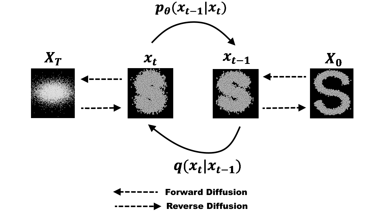
Diffusion models have recently taken the generative AI world by storm, powering state-of-the-art systems like DALL-E 2, Imagen, and Stable Diffusion. Unlike GANs or VAEs, diffusion models work by gradually adding noise to data and then learning to reverse this process.

In this post, we will dive deep into the mathematical foundations of Denoising Diffusion Probabilistic Models (DDPM).

Forward Process (Diffusion)

Main Theory

The forward process, also known as the diffusion process, gradually adds Gaussian noise to a data point sampled from the real data distribution , or over steps, also denoted as .

Each step in the forward process is defined as:

where is a variance schedule and denotes the identity matrix, ensuring that the noise is added independently to each vector dimension.

The formula for adding noise in a single diffusion step is:

This means at each timestep , we generate by blending the previous sample with Gaussian noise scaled by the current variance .

Although it looks like a step-by-step process, a key property of the forward process is that we can sample at any arbitrary time step directly from . Let and . Then:

Or equivalently:

Deriving the Weights: and

We begin with the recurrence relation for the forward diffusion process:

Each follows a standard normal distribution. A key property of normal distributions is that the addition of two independent normal distributions and results in a new normal distribution with mean and standard deviation .

Step-By-Step Expansion

Let’s compute the first few steps to reveal the pattern, applying the rule of adding normal distributions at each step:

• For :
  

• For :
  

  Now we merge the two noise terms and . Since both and are independent , the combined noise is where:
  

  Thus, by writing , we have:
  

• For :
  Following the same logic:
  

  Merging the noise terms again:
  

  So, we have:
  

By induction, we can generalize this pattern for any arbitrary timestep :

where . This powerful result shows that we don't need to iteratively add noise times; we can jump directly from to any in a single calculation.

Intuitive Meaning

• Signal Decay: The original image is gradually “faded out” as it is multiplied by at each step. After steps, the remaining signal is .
• Noise Accumulation: Each step adds a new “layer” of random noise. Because these noise layers are independent, they don't just add up linearly; instead, their variances add up, which is why the total noise standard deviation becomes .
• The Diffusion Limit: As increases towards , approaches 0. This means the original signal eventually vanishes, leaving only pure Gaussian noise.

Variance Schedules

The choice of the variance schedule is crucial for the performance of diffusion models. It determines how quickly the signal is destroyed in the forward process and how much noise the model needs to remove at each step of the reverse process.

Linear Schedule

The linear schedule, introduced in the original DDPM paper, defines as a linear interpolation between two values (typically and ):

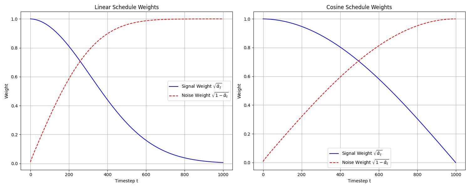
While simple, the linear schedule tends to destroy the signal very quickly in the later steps, which can make the reverse process more difficult to learn.

Cosine Schedule

To address the rapid signal decay of the linear schedule, the cosine schedule was proposed in “Improved Denoising Diffusion Probabilistic Models”. It defines directly using a cosine-based function:

where is a small offset (typically ) to prevent from being too small at . This schedule results in a much smoother decay of the signal, preserving more information for a longer period during the forward process.

The following plots compare the signal weight () and noise weight () for both the linear and cosine schedules.

Reverse Process (Generative)

The goal of a diffusion model is to reverse the forward process. If we can successfully sample backwards from to , we can start from pure Gaussian noise and iteratively denoise it to generate a brand-new, high-quality image .

Using Bayes' formula, the expression of the true reverse conditional probability is:

This is intractable (impossible to compute directly) because the expression of (as well as ) is:

where the distribution of all real images in the world is:

is known. However, is the distribution of all possible clean images . requires integrating over the entire real data distribution, which is infinitely complex. Even if we try to approximate with a lot of real image samples, the amount of calculation needed is impractical since the dimension of is huge (e.g. the dimension is if the image has size ).

To solve this, we train a neural network to approximate this intractable reverse step:

Our main challenge now is: how do we find the training target for the network's predicted mean and variance ?

The Mathematical Trick: Conditioning on

Although is intractable, it becomes surprisingly tractable if we condition it on the original clean image . Think of this as a “cheat code”—if the model knows what the final clean image looks like, calculating the exact reverse step becomes straightforward.

Using Bayes' rule, we can rewrite this conditional probability as:

Notice that every single term on the right side of the equation is a forward process probability that we already defined in the previous section.

• is just the standard one-step forward transition , which is .
• is the “shortcut” transitions that let us jump directly from , which is .
• is similar to above, which is .

The probability density function (PDF) of normal distribution is .

Multiplying these Gaussian densities together, the exponent part of is:

We want the exponent to be in the form of this:

Derive Expression of and

Since is the variable, we will consider everything else as constant, including .

Constant can be removed from the exponent because where is a constant coefficient and does not affect mean and std.

Expand everything and combine:

Now we have this form in the exponent:

where

After removing , we have this form:

So:

Take the inverse:

Similarly:

Finally, we find that is also a Gaussian distribution:

Making Sense of the Ground-Truth Mean

Don't be intimidated by these heavy coefficients! The physical meaning of is beautifully intuitive. It tells us that the best guess for the previous image is a weighted average of two things:

1. The current noisy image .
2. The final clean image .

Shifting from Image Predictor to Noise Predictor

Ideally, we want our neural network's to match the ground-truth mean as closely as possible. However, during real generation, the network does not have access to the clean image .

To bypass this, we use the forward shortcut formula we derived earlier to express in terms of and the actual added noise :

If we substitute this definition of back into the complex equation above, a gorgeous simplification happens after the algebra settles:

Look at this elegant result! The only unknown variable left in this ground-truth mean is —the random noise that was added at timestep .

This reveals the core breakthrough of the DDPM paper: instead of training the neural network to predict the entire complex image mean , we can train it to be a simple noise predictor with a simple MSE loss function:

Sampling Process (Inference)

Basic

Now that our neural network has been trained to predict the noise injected at any given timestep, how do we actually use it to generate a brand-new image?

We start from pure Gaussian noise and run the reverse process step-by-step from down to .

At each reverse step, we want to sample from the predicted distribution .

Using the mathematical breakthrough we derived in the previous section, we can parameterize the network's predicted mean by replacing the true unknown noise with our network's prediction :

For the standard deviation , DDPM sets it as a fixed constant, choosing either of the following (the second one produces a more accurate approximation):

We sample a random noise vector at each step to ensure generation diversity. The final sampling formula for a single reverse step is:

Note on the final step: When , we are generating the final clean image . At this last step, we no longer add random noise, so we set to get the clean deterministic output.

Practical Implementation

Using the sampling process above, the result will be unstable. This is mainly caused by the term.

When the sampling process starts, the first if using cosine scheduler with default parameters. It causes which makes the value of completely off track.

Besides, the value of the term is also unstable. When the process is close to end, , causing the noise weight to explode.

Therefore, we will do the following sampling steps.

First, approximate the clean image by the predicted noise:

Then clip the value to a valid range (usually for pixel values):

Finally, inject the clipped predicted clean image back to the original mean formula to get a more stable result.

Conclusion

The genius of DDPM lies in avoiding the direct calculation of the intractable real data distribution . Instead of forcing a neural network to model a highly complex, multi-modal image manifold all at once, Bayes' rule allows us to break down the task into tiny, tractable, Gaussian-distributed denoising steps.

By shifting the training objective from “predicting a perfect clean image” to “predicting a standard normal noise vector ”, the model transforms a daunting generative task into a stable, iterative regression problem.

With these foundational math formulas locked down, we are now fully equipped to implement this elegant system in PyTorch from scratch!